

What if you could steer the output of a video generation model the way you adjust brightness on your phone? Not by retraining, not by rewriting prompts just by nudging a vector in the model's internal representation. That idea, which made GAN-based image editing almost magical a few years ago, is what drove us to probe the latent space of LTX-2 [5], a modern video diffusion model. The question is deceptively simple: do the same geometric intuitions that made StyleGAN so editable transfer to the latent spaces of diffusion-based video models?
What we found is genuinely interesting not because everything worked, but because what specifically did and didn't work draws a precise map of the latent geometry, and that map points directly toward approaches that should work better. This post walks through the math, the measurements, and what they reveal.
The Geometric Intuition: Linear Directions in Latent Space
In the GAN era, one of the most striking discoveries was that a model's learned latent space often contains linear directions tied to human-understandable concepts. GANSpace [1], InterFaceGAN [2], and related work showed that you could apply PCA or supervised probes to find axes in StyleGAN's [3] space that correspond to "age," "smile," or "lighting angle" and that these directions generalized cleanly across identities. The reason this works is architectural.
A StyleGAN generator has two stages: a mapping network and a synthesis network . The key discovery of GANSpace [1] and InterFaceGAN [2] is that — not — is where semantic directions are most linearly separable.
Since the generator's only learned input is the latent, the systematic axes of visual variation must be organized inside the latent spaces (StyleGAN's per-layer Gaussian noise contributes stochastic detail like hair strands and pore textures, but the semantic content sits in and ). The reason is more linearly disentangled than is architectural: is forced to be Gaussian, but real data is not, and the non-linear mapping network lets adopt a non-Gaussian distribution that follows the data manifold. That distribution-matching is what makes linear arithmetic in produce semantically coherent edits.
LTX-2 [4][5] works differently. Its full architecture is an asymmetric dual-stream rectified-flow transformer that jointly generates video (14B parameters) and audio (5B parameters) with bidirectional cross-attention between the two streams; for this study we ignore the audio stream and probe only the video VAE and the video latent. The architecture follows the latent diffusion paradigm [7], separating the compression step from the generation step. The video VAE encoder takes a full video and compresses it:
The encoder maps this to a compact latent tensor:
LTX-2's VAE applies spatial compression (, ) and temporal compression (, owing to a causal design where the first frame is encoded as a separate latent frame), with latent channels. A 25-frame 544×960 clip compresses to a latent — roughly the size of the original video (the asymptotic per-token ratio is 1:192; the causal "+1" frame makes short clips slightly less compressed).
The generation side is a rectified-flow [6] model: it learns a velocity field that transports samples from pure noise to clean data via ODE integration, rather than the discrete stochastic denoising chain of DDPM-style diffusion. The diffusion transformer operates on , not .
The central question: the GAN's is organized by semantic pressure; the VAE's is organized by compression efficiency. Are those the same thing?
Experimental Setup
The diagram below shows the full LTX-2 pipeline with the intervention point for our study highlighted:
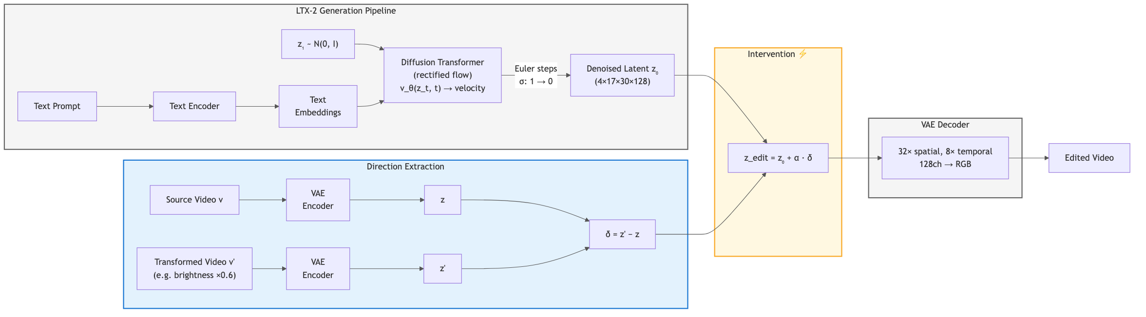
We tested the most direct hypothesis for direction-based editing: encode a video, apply a known pixel-space transformation, re-encode, and take the difference vector in latent space as a candidate semantic direction.
where has a known pixel-space operation applied (e.g., brightness scaled by ). The hypothesis is that is a reusable direction: apply it to any other video's encoding and the same visual transformation should appear.
To test this, we generate a video through the full diffusion process (integrating the learned velocity field from to ), then inject the direction post-hoc:
where is a scalar strength parameter: recovers unchanged, applies the full magnitude of the original difference vector, and larger values extrapolate beyond it. If the latent space has linear semantic structure, sweeping from to should smoothly move the output along the intended transformation axis. The upper bound is an empirical ceiling: beyond it, the decoder receives a latent far outside its training distribution and produces artifacts.
Experimental parameters:
| Parameter | Value |
|---|---|
| Source videos | 4 |
| Directions tested | brightness (factor=0.6), contrast (factor=1.25), grayscale, zoom (scale=1.1), random (control) |
| Alpha sweep | −2.5 to +2.5, 10 values |
| Total samples | 200 (40 per direction) |
| Diffusion steps | 8 |
| Guidance scale | 1.0 |
| Edit injection point | Post-diffusion latent () |
The random direction is the essential control: a tensor sampled from and rescaled so its L2 norm matches that of the transformation direction it's being compared against. It separates "this direction moves the output" from "any direction of this magnitude moves the output."
Here's one of our source videos alongside its pixel-space reference transformation:
| Original source video | Reference: brightness darkened in pixel space |
What the Experiments Revealed
A measurable and structured asymmetry across transformation types
The mean pixel-level metrics across all 40 samples per direction reveal a clear and non-trivial pattern:
| Direction | Mean MAE | Mean MSE | Mean L2 |
|---|---|---|---|
| Brightness | 0.0422 | 0.00806 | 494.8 |
| Contrast | 0.0160 | 0.00175 | 222.4 |
| Random | 0.0105 | 0.000848 | 155.9 |
| Grayscale | 0.0081 | 0.000411 | 108.2 |
| Zoom | 0.0071 | 0.000459 | 111.8 |
All metrics are computed between the edited and unedited output across all pixels and frames. A MAE of means the average edited pixel differs by about of the full pixel range from the original. MSE being higher for brightness than random (while MAE is only higher) tells us brightness-directed edits contain large, localized deviations, not just uniform small shifts. The L2 ratio of vs — a gap in total video-space distance — confirms this at aggregate scale.
What is striking about the table is not just the top it is the bottom. Grayscale and zoom directions score below the random baseline in every metric. A structurally derived direction computed from a deterministic, repeatable pixel-space transformation produces less change than random noise at the same magnitude. This is a precise geometric finding: the latent displacement corresponding to grayscale conversion or zoom is, when applied to a different video's latent neighborhood, nearly orthogonal to the directions that move the decoder output at all. The brightness direction, by contrast, consistently outperforms random telling us that brightness differences project into latent space with more transfer-relevant geometry than grayscale or zoom differences do.
The spatial structure of changes is informative
When we apply the brightness direction at and amplify the pixel difference by , the diff video doesn't show uniform darkening it shows spatially structured colour redistribution concentrated at high-contrast regions and dominant colour areas.
| Brightness direction applied (α=2.0) | Difference from original (amplified 20×) |
This spatial structure is itself a finding. A truly random latent perturbation decodes to spatially uncorrelated noise. The fact that the brightness direction produces spatially structured changes following image content rather than being uniform means the latent space does encode spatial structure that the decoder respects. The direction is influencing the decoder's reconstruction in content-aware ways; it is just not doing so along the semantic axis we aimed for. Understanding what axis it is following is a productive next question.
Alpha reveals the decoder's response curve
Sweeping from to produces a monotonically increasing relationship between and all three metrics. This is meaningful: it confirms the direction vectors are genuine geometric objects in latent space, not noise. A direction that had no relationship to the decoder's output would show flat or chaotic metric response across the sweep we do not see that.
What the sweep also shows is that the character of the change does not evolve toward the intended transformation as grows. The distortion scales in magnitude but not in semantic specificity. Plotting MAE against for the brightness direction gives a smooth, near-linear curve which is exactly the behavior of moving along a direction in a locally linear space. The latent space is locally linear in the region we are exploring; the issue is that the direction we chose does not align with the semantic axis of brightness. This distinction matters for what to try next.
Transfer behavior maps the local manifold geometry
A direction computed from one source video applied to three other videos shows inconsistent metric responses some videos react strongly, others weakly, with no pattern tied to visual similarity or content type. This is a structural observation about the local geometry of the latent manifold: the neighborhood around each video's encoding has different curvature and different alignment with the global direction vector. What looks like a meaningful direction near one encoding can be nearly orthogonal to the decodable directions near another.
This non-uniformity is precisely what motivates moving from single-sample difference vectors to corpus-level direction discovery methods the right direction is likely one that is consistently decodable across many local neighborhoods, not just one.
What the Latent Geometry Tells Us
To understand why different transformations produce such different results, it helps to look at what the VAE's training objective actually optimizes. The VAE loss combines five terms:
Pixel reconstruction (MSE):
Direct pixel-level accuracy across all pixels and frames. Squaring penalizes large per-pixel deviations heavily, ensuring the decoded video closely tracks the original.
Video-DWT loss: To ensure reconstruction of high-frequency details that pixel-level MSE tends to miss, an L1 loss is computed across the 8 subbands of a 3D Discrete Wavelet Transform (the tensor-product subbands LLL, LLH, …, HHH) applied to the input and reconstructed videos. This explicitly penalizes blurred or smeared spatiotemporal detail.
Perceptual loss (LPIPS):
LPIPS [8] sums across multiple layers of a pretrained feature network, with features unit-normalized along the channel axis and weighted per-channel by learned scalars . This compares structured perceptual features rather than raw pixels, encouraging textures, edges, and structure to match without requiring exact pixel-level agreement.
Reconstruction-GAN loss: Unlike a standard PatchGAN, the discriminator here receives the original and reconstructed videos as a concatenated pair and is trained to identify which of the two is the original. The relative comparison actually simplifies the discriminator's job — D no longer has to model the full distribution of real videos, only spot which sample in the pair is the source — and a stronger, better-calibrated D in turn forces the decoder toward reconstructions that match the source faithfully rather than ones that just look generically realistic.
KL divergence regularization:
The encoder outputs parameters of a Gaussian , with a single log-variance shared across all latent channels. Minimizing pulls each video's posterior toward the prior, which keeps the aggregate posterior overlapping the standard normal — so the decoder sees a consistent latent distribution at training and inference time.
Crucially, none of these five terms reward the latent for organizing semantic concepts along separable linear axes. They reward accurate reconstruction, frequency fidelity, perceptual similarity, realism, and distributional regularity. The latent that minimizes this objective is one that encodes videos efficiently not one that places "brightness" along one axis and "contrast" along another.
This is the key architectural distinction from a GAN. In a GAN, the latent spaces ( and ) are the only source of semantic variation, so semantic structure is forced into them. In LTX-2, semantic variation is handled by the diffusion transformer a separate, much larger network that operates on conditioned on text prompts via cross-attention. The VAE's job is purely compression.
This is why the specific difference vector
carries only partial signal. The element-wise difference captures the total response of every convolutional filter to the brightness change — including brightness-correlated frequency components (explaining the above-baseline MAE) but also histogram shape, local contrast ratios, edge detector responses, and normalization layer statistics. All of this ends up entangled in .
Grayscale and zoom show a different and equally informative pattern. Grayscale conversion removes chrominance while preserving luminance structure. Zoom resamples spatial positions. Both of these transformations produce latent differences that, when applied to a new video, are nearly orthogonal to the directions the decoder is sensitive to — moving along barely perturbs the decoded output, so the metrics fall below even an isotropic random perturbation of the same magnitude. That is a quantitative property of the latent manifold geometry, not just a null result: the encoder's response to grayscale or zoom in one video lies in a subspace that, around other videos' encodings, the decoder essentially ignores.
The temporal axis compounds this. has shape . Adding applies the same displacement uniformly across all time positions every frame gets shifted by the same latent-space amount simultaneously. There is no temporal selectivity, no per-frame adaptation. The decoder must then reconstruct a video that is temporally consistent from a latent that was shifted in a direction agnostic to temporal relationships. This is structurally harder than the static-image case and is why video latent editing is a meaningfully different problem from image latent editing.
Where This Points
Each finding above is a constraint on the search space, and constraints are useful. Here is what they motivate.
Corpus-level direction discovery. The single-pair difference vector is a sample of size one from the distribution of brightness-induced latent differences. A more robust approach computes this for thousands of pairs:
and then extracts the principal components of this distribution. The first principal component of is the direction that explains the most variance in how brightness transformations move latents a direction that generalizes across local neighborhoods rather than overfitting to one. This is exactly the logic behind GANSpace, and it transfers directly to this setting.
Supervised linear probing on encoder internals. The encoder is not a black box it is a sequence of convolutional layers, each producing an intermediate feature map. Training a linear classifier on these intermediate activations to predict the transformation label (bright / dark / grayscale / etc.) gives a probe whose weights are, by construction, the most linearly separable direction for that property at that layer. These weights are candidate directions that have been explicitly optimized for semantic alignment, rather than derived from the decoder's reconstruction geometry.
Editing inside the diffusion transformer. The semantic structure we are looking for exists in the model it must, because the model generates visually coherent content conditioned on semantic text descriptions. That structure lives in the diffusion transformer's activations, particularly in the self-attention patterns and cross-attention maps at specific denoising timesteps . At early timesteps ( near ), the model operates on highly noisy latents and makes coarse structural decisions; at late timesteps ( near ), it refines fine details. Targeted interventions at specific timesteps adding a displacement in the transformer's activation space rather than in would propagate through the remaining denoising steps with the model's semantic priors intact.
Noise-space perturbation. Rather than editing the final denoised latent , we can perturb the starting noise before the reverse process begins. LTX-2 is a rectified-flow model: the forward process linearly interpolates between data and noise as , and the network is trained to predict the velocity , i.e., minimizing . Generation integrates this velocity field from (pure noise) to (clean data) via an ODE solver. In practice, an Euler step suffices:
where decreases from (pure noise) to (clean data) over the sampling schedule. A perturbation in flows through all steps of this integration, each involving a semantic velocity prediction by . Rather than a single post-hoc latent shift, the edit participates in every denoising step giving the model's learned velocity field the opportunity to interpret and amplify the perturbation coherently across the full generation process.
Key Takeaways
We set out to map the geometric structure of LTX-2's VAE latent space through a controlled set of direction-discovery experiments. The measurements are informative in ways that point well beyond this initial probe.
The asymmetry across transformation types is a finding, not a null result. Brightness-derived directions outperform the random baseline by in MAE. Grayscale and zoom directions fall below the random baseline. This is a quantitative statement about which transformation types have latent geometry that transfers across video encodings and which do not and it is the kind of constraint that should inform which transformations are productive targets for more sophisticated direction-discovery methods.
The spatial structure of decoder responses confirms content-aware latent encoding. The diff videos show spatially structured changes concentrated at content-relevant regions, not uniform noise. This means the latent space genuinely encodes spatial information that the decoder uses the opportunity for content-aware editing is real; the method just needs to find directions aligned with semantically meaningful axes.
The -sweep response curve confirms local linearity. Monotonic, near-linear MAE response to means the latent space is locally linear in the explored region. Linear editing should work here the question is whether the directions we compute point in the right places in that linear space.
The architectural separation between compression and semantics is the key insight. The VAE's training objective does not create semantic axes but that does not mean the latent lacks structure. It means the structure present is compression-optimal, and extracting semantically aligned directions from it requires methods (corpus PCA, supervised probing, contrastive optimization) designed to find those aligned directions rather than naively reading off single-sample differences.
The semantic structure that makes video generation possible is distributed across the diffusion transformer's learned weights and attention patterns. Finding a way to access it through the VAE latent, through the transformer's activations, or through the noise space is the next and genuinely open question. These experiments give us a precise starting point.
References
[1] Härkönen, E., Hertzmann, A., Lehtinen, J. and Paris, S., 2020. Ganspace: Discovering interpretable gan controls. Advances in neural information processing systems, 33, pp.9841-9850.
[2] Shen, Y., Gu, J., Tang, X. and Zhou, B., 2020. Interpreting the latent space of gans for semantic face editing. In Proceedings of the IEEE/CVF conference on computer vision and pattern recognition (pp. 9243-9252).
[3] Karras, T., Laine, S. and Aila, T., 2019. A style-based generator architecture for generative adversarial networks. In Proceedings of the IEEE/CVF conference on computer vision and pattern recognition (pp. 4401-4410).
[4] HaCohen, Y., Chiprut, N., Brazowski, B., Shalem, D., Moshe, D., Richardson, E., Levin, E., Shiran, G., Zabari, N., Gordon, O., Panet, P. et al., 2025. Ltx-video: Realtime video latent diffusion. arXiv preprint arXiv:2501.00103.
[5] HaCohen, Y., Brazowski, B., Chiprut, N., Bitterman, Y., Kvochko, A., Berkowitz, A., Shalem, D., Lifschitz, D., Moshe, D., Porat, E., Richardson, E. et al., 2026. LTX-2: Efficient Joint Audio-Visual Foundation Model. arXiv preprint arXiv:2601.03233.
[6] Liu, X., Gong, C. and Liu, Q., 2022. Flow straight and fast: Learning to generate and transfer data with rectified flow. arXiv preprint arXiv:2209.03003.
[7] Rombach, R., Blattmann, A., Lorenz, D., Esser, P. and Ommer, B., 2022. High-resolution image synthesis with latent diffusion models. In Proceedings of the IEEE/CVF conference on computer vision and pattern recognition (pp. 10684-10695).
[8] Zhang, R., Isola, P., Efros, A.A., Shechtman, E. and Wang, O., 2018. The unreasonable effectiveness of deep features as a perceptual metric. In Proceedings of the IEEE Conference on Computer Vision and Pattern Recognition (pp. 586-595).