*Part 4 of 4 — Distributed Training series. Start with the overview.*

1. Distributed Data Parallel: How It Actually Works — Scale throughput when the model fits on one GPU. 2. ZeRO and FSDP: Model Sharding — Fit models that don't fit, by sharding weights, gradients, and optimizer state. 3. Tensor Parallelism and Sequence Parallelism — Shard inside each layer; wins when interconnect is slow or a single layer is oversized. 4. Pipeline Parallelism: How It Actually Works (this post) — Shard across layers; the axis that cheaply spans nodes.

Most distributed training strategies have one thing in common: every GPU holds the full set of layers. → DDP replicates the entire model on each rank. → FSDP shards each weight tensor but every rank still walks the same layer list during forward and backward. → TP shards inside each layer but every rank participates in every layer. The unifying assumption across all of them is that "the model", every parameter and every activation slot, is something each rank has *some view of*.

Pipeline Parallelism breaks that assumption. With PP, rank 0 holds the first N/2 layers. Rank 1 holds the next N/2. Rank 0 has never seen rank 1's weights and never will. The forward pass is no longer a single rank running 36 decoder layers; it is rank 0 running its 18 layers, sending the resulting hidden state across the network to rank 1, and rank 1 running the other 18.

This is the parallelism strategy you reach for when the model itself is too large for one GPU. A 70B BF16 model is 140 GB of weights, and even with FSDP sharding it across 8 cards, the per-GPU footprint is ~17.5 GB just for parameters, before activations or optimizer state. PP solves the same problem differently: instead of distributing every parameter across every GPU, it distributes *which layers live where*. Each GPU only sees its own slice and never has to gather the full weight matrices.

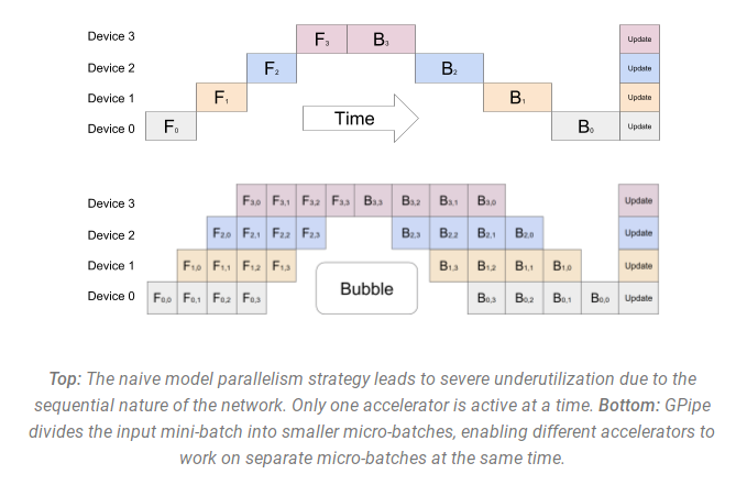
!GPipe pipeline parallelism bubble *Naive model parallelism (top) vs GPipe pipeline parallelism with microbatches (bottom). The grey region is the bubble. Source: HuggingFace transformers parallelism docs, originally from the GPipe paper.*

The cost of this is a phenomenon that doesn't exist in any of the other strategies: the pipeline bubble, the idle time when one rank is waiting on another. The whole intellectual content of pipeline parallelism is the techniques that shrink the bubble. Microbatching, schedule design, the difference between GPipe and 1F1B, interleaved schedules: these are not implementation details. They are the entire reason PP is interesting.

This post walks through how PP partitions a transformer, where the bubble comes from, why microbatching shrinks it, what 1F1B actually does compared to GPipe, and what the trade-offs look like in practice. The reference implementation is experiments/pp-ft/train.py, which uses PyTorch's native torch.distributed.pipelining API to finetune Qwen3-4B with LoRA on the AMI meeting transcript dataset (knkarthick/AMI) on 2x RTX 4090.

---

Why You Reach For Pipeline Parallelism

Each of the four common parallelism strategies solves a different problem.

| Strategy | Solves | Cost | |---|---|---| | → DDP | Throughput. Model fits on 1 GPU; you want to train faster. | None except gradient AllReduce overhead. | | → FSDP | Memory. Model nearly fits on 1 GPU; sharding parameters/grads/optimizer states gets you the rest of the way. | AllGather + ReduceScatter per layer. | | → TP | Compute inside a layer. The matmuls themselves are large enough that splitting them across GPUs is faster than running them sequentially. | AllReduce per row-parallel boundary, very latency-sensitive. | | PP | The model literally doesn't fit on 1 GPU, even sharded. | The pipeline bubble: idle time inherent to streaming activations between stages. |

PP is the strategy where the failure mode without it is "the program doesn't run," not "it runs slowly." If → FSDP can shard a model into a working configuration, you should use FSDP. If → TP can split the matmul tensors so they fit, you should use TP. PP is what you do when neither of those is enough.

"Neither of those is enough" is more specific than it sounds. → TP requires NVLink-class bandwidth on every per-layer AllReduce, which caps it at around 8 GPUs (one DGX or HGX node). You cannot do TP=64 across nodes because InfiniBand isn't fast enough. → FSDP's roughly 3x-model-size weight traffic per step becomes bandwidth-bound past a certain world size, and activation memory still grows with batch * seq * hidden * num_layers regardless of how well parameters are sharded.

PP is the only axis that drops activation memory by 1/stages, communicates just one hidden-state tensor per microbatch (cheap enough to cross nodes), and composes orthogonally with DP, FSDP, and TP. In the large pretraining stacks it shows up as the *outer* axis: TP inside the node, FSDP or DP across replicas, PP across pipeline stages that span nodes.

Every dense model above 100B parameters is trained this way:

| Model | Parallelism layout | |---|---| | GPT-3 175B | TP=8 x PP=16 x DP=many (Megatron-LM) | | PaLM 540B | Same conceptual layout on TPU pods | | Llama-3 405B, Mixtral, DeepSeek-V3 | PP as one axis in their respective stacks |

The production frameworks that implement PP include Megatron-LM, DeepSpeed (PipelineModule), NVIDIA NeMo, PyTorch's torch.distributed.pipelining (what this experiment uses), Google's T5X/Pax/MaxText on TPU, HuggingFace nanotron, and Colossal-AI.

When you actually need PP: under 30B you almost never do. Between 30B and 70B you can usually avoid it with FSDP+TP if your interconnect is good. Beyond roughly 100B parameters or very long context, PP becomes structurally unavoidable.

For Qwen3-4B on a 24 GB GPU, PP is overkill. The model fits comfortably. The reason this post uses a 4B model anyway is to make the mechanics visible at a scale you can actually run on two consumer cards. The numbers from the run are honest about that: PP at 4B is a teaching demo, not a production fit. The interesting part is the structure, which generalizes directly to the scales where PP becomes essential.

---

How PP Splits a Model

A transformer is a stack of identical decoder layers, sandwiched between an embedding lookup at the start and a normalization + language model head at the end. PP slices that stack along its depth.

For Qwen3-4B with 36 layers and PP degree 2:

` Rank 0 (stage 0): Rank 1 (stage 1): embed_tokens layers[18] layers[0] layers[19] layers[1] ... ... layers[35] layers[17] norm lm_head `

Each rank holds exactly the parameters for its own slice and nothing else. Stage 0 is responsible for turning input token IDs into a hidden state at the boundary between layer 17 and layer 18. Stage 1 takes that hidden state, runs it through layers 18-35, applies the final norm, projects to the vocabulary, and produces logits.

The communication is point-to-point and trivial: rank 0 sends one tensor of shape [batch, seq, hidden] to rank 1 during the forward pass, and rank 1 sends a gradient tensor of the same shape back to rank 0 during the backward pass. There are no AllReduces, no AllGathers, no ReduceScatters. PP is the only common parallelism strategy whose cross-rank communication is just send/recv. Every other strategy uses collective operations across all ranks at once.

This sounds great until you draw the timeline.

---

The Pipeline Bubble

Here is what one forward and one backward pass look like with no microbatching:

` time ────────────────────────────────────► rank 0: [F0] [B0] rank 1: [F1] [B1] `

Rank 0 runs its forward, sends the hidden state to rank 1, then sits idle. Rank 1 runs its forward, computes the loss, runs its backward, and sends the input gradient back to rank 0. Then rank 0 runs its backward.

The amount of idle time on each rank is *50% of the total step*. Doubling your GPU count halved the work per GPU, but it also halved the utilization. The total wall-clock time is roughly the same as running the whole thing on one GPU, except you spent twice the hardware to do it.

This is the bubble. It comes from one fact: stage 1 cannot start until stage 0 finishes, and stage 0 cannot start its backward until stage 1 finishes. The dependencies are sequential, and any sequential chain in a parallel system is dead time on every rank that isn't currently the active link.

The bubble is the central problem of pipeline parallelism. Every named technique in PP, microbatching, GPipe, 1F1B, interleaved schedules, looped BFS, exists to make it smaller.

---

Microbatching

The first move is to notice that the bubble exists because we treated the batch as one indivisible unit. If we split the batch into N microbatches, rank 0 can start working on microbatch 2 as soon as it finishes microbatch 1, even though rank 1 is still busy with microbatch 1.

` time ─────────────────────────────────────────────────► rank 0: [F0₁][F0₂][F0₃][F0₄] [B0₁][B0₂][B0₃][B0₄] rank 1: [F1₁][F1₂][F1₃][F1₄] [B1₁][B1₂][B1₃][B1₄] `

This is GPipe (Huang et al., 2018). All forward microbatches happen first on every rank, then all backward microbatches happen, in reverse microbatch order. The pipeline fills, runs at full capacity for most of the step, and drains.

The bubble shrinks because the fill and drain are now a smaller fraction of the total work. With nmicrobatches microbatches and numstages stages, the bubble fraction is:

` bubble = (numstages - 1) / (numstages - 1 + n_microbatches) `

For 2 stages and 8 microbatches: 1 / (1 + 8) = 11%. For 4 stages and 16 microbatches: 3 / (3 + 16) = 16%. The pattern is clear: more microbatches help, but with diminishing returns. Past a certain point, the per-microbatch overhead (Python dispatch, kernel launch latency, send/recv overhead) starts dominating the savings.

There is also a memory cost. GPipe holds *all* microbatches' activations in memory simultaneously on every rank, because the backward pass for microbatch 1 depends on the forward activations from microbatch 1, and those have to survive until the backward starts. With 8 microbatches the activation memory is 8x what it would be without microbatching. For a 4B model on a 24 GB GPU this is fine; for a 70B model on 80 GB it can become the limiting factor.

---

1F1B: One Forward, One Backward

The fix to GPipe's memory cost is 1F1B (one-forward-one-backward), the schedule used by Megatron-LM and most production stacks. The idea: once the pipeline is filled, every rank alternates one forward microbatch with one backward microbatch. The backward is from an *earlier* microbatch whose forward has already completed, so its activations can be freed as soon as the backward finishes.

` time ──────────────────────────────────────────────────► rank 0: [F0₁][F0₂][F0₃][F0₄][B0₁][F0₅][B0₂][F0₆][B0₃][F0₇][B0₄] ... rank 1: [F1₁][F1₂][F1₃][B1₁][F1₄][B1₂][F1₅][B1₃][F1₆][B1₄] ... `

(Schematic; the exact ordering depends on the schedule's startup phase.)

The bubble fraction is the same as GPipe: both are (N-1)/(N-1+M) for N stages and M microbatches, because the fill and drain are unchanged. The win is memory: peak activation memory drops from M microbatches per rank to roughly 2 * num_stages microbatches per rank, and the constant factor is small. Concretely, for 8 microbatches on 2 stages, GPipe holds 8 microbatches' activations and 1F1B holds about 4. For 16 microbatches on 4 stages, GPipe holds 16 and 1F1B holds about 8. As you scale microbatches up (which is what you want for a smaller bubble), GPipe's memory grows linearly while 1F1B's stays bounded.

To anchor that in real numbers: each microbatch stores the hidden state at every layer boundary for backward. For Qwen3-4B with PP=2, each stage has 18 layers, and one microbatch's stored activations are roughly 18 layers * [1, 512, 2560] * 2 bytes = ~47 MB. GPipe holding 8 microbatches costs ~380 MB; 1F1B holding 4 costs ~190 MB. The difference is under 200 MB -- negligible at 4B scale, which is why our run fits comfortably either way. At 70B the math changes: hidden_size=8192, seq=4096, PP=8 with 10 layers per stage, and 32 microbatches. GPipe holds ~21 GB of activations per rank; 1F1B holds ~10 GB. On an 80 GB A100, that 11 GB gap is the difference between fitting and not fitting.

This is why every modern pipeline schedule descends from 1F1B. PyTorch's torch.distributed.pipelining ships Schedule1F1B as its standard non-interleaved option, alongside ScheduleGPipe (kept for pedagogical contrast) and ScheduleInterleaved1F1B (a variant we'll get to in a moment).

---

Interleaved 1F1B

There is one more lever. The bubble formula (N-1)/(N-1+M) gets smaller as you add microbatches (good), but it also gets *bigger* as you add stages (bad). For a deep pipeline of, say, 8 stages, even M=32 microbatches still leaves you with a 7/(7+32) ≈ 18% bubble.

Interleaved 1F1B (Megatron's "virtual pipeline parallelism") fixes this by giving each rank multiple non-contiguous slices of the model instead of one contiguous slice. With 8 ranks and virtualpipelinesize=2, each rank holds 2 separate "model chunks": rank 0 gets layers [0:5] and [40:45], rank 1 gets [5:10] and [45:50], and so on. The pipeline now has 8 * 2 = 16 virtual stages, which reduces the bubble fraction by a factor of 2 at the cost of doubling the number of point-to-point sends per microbatch.

` time ─────────────────────────────────────────────────────────► rank 0: [F0a₁][F0b₁][F0a₂][F0b₂][B0a₁][F0a₃][B0b₁][F0b₃][B0a₂][F0a₄] ... rank 1: [F1a₁][F1b₁][F1a₂][B1a₁][F1b₂][B1b₁][F1a₃][B1a₂][F1b₃] ... `

(F0a₁ = stage 0, chunk a, microbatch 1. Each rank juggles two model chunks. The bubble shrinks because the interleaving lets ranks overlap fill and drain across chunks: the bubble is still (p-1) time units, but each rank now does v * M units of useful work instead of M. The effective bubble fraction becomes (p-1) / (p-1 + v*M) -- for 8 ranks, v=2, M=32: 7/71 ≈ 10% vs 7/39 ≈ 18% without interleaving.)

Interleaved 1F1B is what large training runs at companies like Meta, Google, and NVIDIA actually use. It's also more complex to schedule and reason about. PyTorch's ScheduleInterleaved1F1B exposes it; the reference implementation in this post uses plain Schedule1F1B because at PP=2 the interleaved variant doesn't help.

---

The PyTorch API

PyTorch's torch.distributed.pipelining (stable since torch 2.4, formerly torch.distributed.pipeline.sync and before that the standalone PiPPy library) is the modern answer for PP. It does three things:

1. PipelineStage wraps a per-rank nn.Module and tracks the metadata the schedule needs: the stage index, the total number of stages, the device, and the forward signature. 2. Schedule1F1B (or ScheduleGPipe, or ScheduleInterleaved1F1B) takes a PipelineStage and a microbatch count and exposes a step() method that drives the pipeline. 3. The schedule's step() accepts the input on stage 0, the target labels on the last stage, and a list to capture per-microbatch losses. Internally it splits the input along the batch dimension, sends and receives hidden states between adjacent ranks via dist.send/dist.recv (under the hood), and orchestrates the schedule.

The minimum viable PP training loop looks like this:

`python from torch.distributed.pipelining import PipelineStage, Schedule1F1B

Each rank builds its own stage_module: a plain nn.Module that knows how to

forward over its slice of the layers.

stagemodule = buildstageforthisrank(rank, worldsize)

stage = PipelineStage( stage_module, stage_index=rank, numstages=worldsize, device=torch.device(f"cuda:{local_rank}"), )

def loss_fn(logits, labels): shift_logits = logits[:, :-1, :].contiguous() shift_labels = labels[:, 1:].contiguous() return F.cross_entropy( shiftlogits.view(-1, shiftlogits.size(-1)).float(), shift_labels.view(-1), ignore_index=-100, )

schedule = Schedule1F1B(stage, nmicrobatches=8, lossfn=loss_fn)

for input_ids, labels in loader: losses_buf = [] if rank == 0: schedule.step(input_ids) elif rank == world_size - 1: schedule.step(target=labels, losses=losses_buf) else: schedule.step() optimizer.step() optimizer.zero_grad() `

A few things to notice:

Stage 0 calls schedule.step(input). Only the first stage takes the raw input, because only it has the embedding table.

The last stage calls schedule.step(target=..., losses=...). Only the last stage has the lm_head, the loss function, and the target labels. The losses list is the API contract: pass it in, and the schedule fills it with one loss tensor per microbatch.

Intermediate stages call schedule.step() with no arguments. They just forward whatever they receive from the previous stage and pass it to the next.

optimizer.step() is called by every rank. Each rank's optimizer only sees its local parameters (its stage's slice), so each rank updates its own piece of the model independently.

The schedule handles all the cross-rank send/recv internally. From the user's perspective, the only thing that distinguishes the PP training loop from a single-GPU one is the rank-conditional schedule.step() call.

---

The Per-Stage Module

The interesting code is what stage_module actually contains. PyTorch's API gives you a lot of flexibility here: you can define any nn.Module with any forward signature, as long as stage 0 takes your raw input, intermediate stages take a hidden state, and the last stage returns whatever the loss function expects.

For Qwen3 the cleanest approach is to mirror what Qwen3Model.forward does internally (embed, run layers, normalize, project) but only over this stage's slice. The per-stage wrapper from experiments/pp-ft/train.py looks like this:

`python class PPQwen3Stage(nn.Module): def _init(self, peftmodel, stageidx, numstages): super()._init_() self.stageidx, self.numstages = stageidx, numstages

inner = peftmodel.basemodel.model.model layersperstage = len(inner.layers) // num_stages start = stageidx * layersper_stage end = start + layersperstage if stageidx < numstages - 1 else len(inner.layers) self.layers = nn.ModuleList(list(inner.layers)[start:end])

self.embedtokens = inner.embedtokens if stage_idx == 0 else None self.norm = inner.norm if stageidx == numstages - 1 else None self.lmhead = peftmodel.basemodel.model.lmhead if stageidx == numstages - 1 else None self.rotaryemb = inner.rotaryemb

def forward(self, x): hidden = self.embedtokens(x) if self.stageidx == 0 else x b, s = hidden.shape[:2] position_ids = torch.arange(s, device=hidden.device).unsqueeze(0).expand(b, -1) positionembeddings = self.rotaryemb(hidden, position_ids)

for layer in self.layers: hidden = layer(hidden, positionids=positionids, positionembeddings=positionembeddings)[0]

if self.stageidx == self.numstages - 1: return self.lm_head(self.norm(hidden)) return hidden `

A few details worth pointing out:

The slicing happens in _init. We grab the full list of decoder layers from the loaded HuggingFace model, take only this stage's slice, and re-wrap them in a fresh nn.ModuleList. The embedtokens lookup is held only by stage 0; norm and lm_head are held only by the last stage. Intermediate stages would hold neither.

The forward signature is forward(x), just one positional argument. PyTorch's pipelining will pass the input here on stage 0 and the previous stage's output here on every other stage. The branch if self.stageidx == 0 decides whether x is inputids (and needs embedding) or a hidden state (and is used as-is).

positionembeddings is a recent addition. Since transformers 4.45, every Qwen3 decoder layer requires positionembeddings=(cos, sin) as a kwarg. We compute it from the model's rotary embedding module on every stage independently. This is not strictly necessary; you could compute it once on stage 0 and ship it down the pipeline, but having each stage recompute its own copy avoids a custom protocol on top of the schedule's send/recv.

attention_mask=None lets PyTorch's SDPA attention infer a causal mask. If you needed to support packed sequences or padding, you'd build the 4D mask here.

The slicing approach has one subtle implication: when we hand peft_model to the constructor, PEFT has already wrapped every target nn.Linear in a LoraLinear. When we then take a slice of inner.layers and put it in a fresh ModuleList, those LoraLinear wrappers come along for free. PEFT's adapter parameters are owned by the layers, not by the top-level model, so slicing the layers slices the adapters. This is the entire reason PP + LoRA "just works": there's no DTensor mismatch, no decoder-layer rewrite, no shape negotiation. The standard PEFT call composes cleanly with the standard PP call.

This is the contrast with → TP: TP needs LoRA to participate in DTensor-aware tensor operations, which the standard PEFT LoraLinear.forward is not built for (see the TP post's "LoRA with TP" and "Why Sequence Parallelism Breaks With LoRA" sections). PP just needs LoRA to live in the layers, which is exactly where PEFT puts it.

---

Reading the Numbers

For Qwen3-4B on 2x RTX 4090 (PCIe, Vast.ai), the PP run lands at:

| Metric | PP (this run) | → DDP (for comparison) | |---|---|---| | Tokens/sec (aggregate) | ~6,950 (steady state) | ~5,800 | | Step time | ~2.36s | ~2.5s | | VRAM per GPU | 4.7 GB | 5.9 GB | | Effective batch size | 16 | 16 | | Sequence length | 512 | 512 | | PP degree / microbatches / schedule | 2 / 8 / 1F1B | -- | | Gradient accumulation | 2 | 8 | | Start loss (epoch 0 step 1) | 3.36 | 3.24 | | End loss (epoch 2 step 45) | 2.47 | ~2.3 | | Total training time | ~110 s (3 epochs) | ~120 s |

Microbatching vs gradient accumulation. These are independent mechanisms that operate at different levels. Microbatching is *inside* a single schedule.step() call: the schedule splits the input batch into M microbatches and streams them through the pipeline to keep all stages busy. Gradient accumulation is *across* multiple schedule.step() calls: gradients from successive steps are summed before the optimizer update. In this run, each schedule.step() processes a batch of 8 samples split into 8 microbatches of 1, and GRAD_ACCUM=2 means two such steps run before optimizer.step(), for an effective batch of 16. DDP achieves the same effective batch size differently: each rank processes 1 sample per forward pass, accumulates over 8 steps, and AllReduce fires on the final step.

Loss drops cleanly from 3.36 to 2.47 over 45 optimizer steps. Two things worth flagging:

PP is slightly faster than DDP here, not slower. Each PP rank only runs half the layers per microbatch, and the ~11% bubble (1/9 at PP=2, M=8) is more than offset by the halved per-microbatch compute. This does *not* generalize: at PP=4 the bubble jumps to 3/11 ≈ 27%, and at larger pipeline depths you need proportionally more microbatches to keep it small.

VRAM is lower because each rank only holds half the model, plus 1F1B caps activation memory at about 2 microbatches per rank. Real, but not the reason you'd choose PP at 4B; DDP fits fine.

The headline is not "PP beats DDP." It is "PP at PP=2 on PCIe is competitive with DDP while using less per-GPU VRAM." On NVLink the send/recv between stages is essentially free, which is why PP scales naturally to deeper pipelines across nodes where TP cannot.

---

The Full Scripts

Two files implement the experiment.

experiments/pp-ft/train.py is about 500 lines in a single file. Loads Qwen3-4B in BF16 on every rank, applies PEFT LoRA, slices out this rank's stage into a PPQwen3Stage, builds a PipelineStage, drives Schedule1F1B with 8 microbatches, broadcasts the loss from the last rank to rank 0 for logging, saves a per-rank LoRA shard at the end of each epoch.

`bash uv sync uv run torchrun --nprocpernode=2 experiments/pp-ft/train.py `

experiments/pp-ft/infer.py is about 150 lines. Each rank saves its own adaptermodel.bin; infer reassembles by remapping the renumbered local layer indices back to global (globalidx = rank * layersperstage + local_idx), merges each LoRA pair into the corresponding base weight, and runs model.generate() on a random AMI test sample.

`bash uv run python experiments/pp-ft/infer.py `

The key takeaway from the script is that PP + LoRA + PyTorch's native pipelining API is genuinely just composing three standard pieces. There is no DTensor mismatch, no decoder layer rewrite, no monkey-patch. The only custom code is the per-stage wrapper module (~50 lines), the broadcast for loss reporting (~5 lines), and the layer-index remapping in the infer script (~10 lines). The rest is stock PyTorch and stock PEFT.

---

Composing PP With Other Strategies

PP is almost never used alone at scale. At 100B+ parameters the pretraining layout typically stacks all four axes together: → TP within a node (NVLink makes per-layer AllReduces cheap), PP across nodes (send/recv tolerates slow inter-node links), and → DDP/→ FSDP across replicas of that TP+PP slice. The assignment follows a principle: map the most latency-sensitive axis to the fastest link.

| Axis | Communication pattern | Maps to | Why | |---|---|---|---| | TP | Many small AllReduces per layer | NVLink (intra-node) | Latency-sensitive: 72+ AllReduces per forward pass | | PP | Point-to-point send/recv between stages | InfiniBand / Ethernet (inter-node) | Latency-tolerant: one hidden-state tensor per microbatch | | DP / FSDP | One AllReduce (or AllGather + ReduceScatter) per step, overlapped with backward | Whatever is left | Bandwidth-sensitive but infrequent |

PyTorch's DeviceMesh is the primitive that makes the composition tractable: it defines the global rank space as a multidimensional grid with named axes, and slicing along an axis gives you exactly the process group that axis's collectives should target.

`python from torch.distributed.devicemesh import initdevice_mesh

8 GPUs arranged as DP=2 x PP=2 x TP=2

mesh = initdevicemesh("cuda", (2, 2, 2), meshdimnames=("dp", "pp", "tp"))

mesh["tp"] # -> TP process groups (for AllReduce inside each layer) mesh["pp"] # -> PP process groups (for send/recv between stages) mesh["dp"] # -> DP process groups (for gradient sync across replicas) `

torch.distributed.pipelining is designed to stack with parallelize_module (TP) and FSDP on top of such a mesh. Production stacks — TorchTitan, Megatron-LM, NeMo — all build on this idea. None of it is required for standard finetuning; this series stops at the single-axis deep dives because at 4B–70B scale one axis is usually enough.

---

When to Use PP

The decision tree is short. Under 30B parameters, you almost never need PP: → DDP handles throughput, → FSDP or → TP handles memory, and the bubble overhead is pure waste at a scale where simpler strategies work. Between 30B and 70B, FSDP+TP on good intra-node interconnect (NVLink) can usually avoid PP entirely. Beyond roughly 100B parameters or very long context, PP becomes structurally unavoidable: TP can't cross node boundaries, FSDP's weight traffic saturates the interconnect, and activation memory grows with depth regardless of how well parameters are sharded. PP is the only axis that cuts activation memory by 1/stages and communicates cheaply enough to span nodes.

This is the last post in the series. → DDP covered throughput scaling, → FSDP covered memory sharding, → TP+SP covered intra-layer parallelism. PP completes the picture by splitting the model along its depth — the axis you reach for last, when nothing else can cross a node boundary.